

What Is Signal Integrity in 5G PCB Design?
Signal integrity in 5G PCB design means one thing: ensuring that high-speed signals travel across the board and arrive clearly and intact—free from distortion, loss, or interference.
The move to 5G, with frequencies from sub-6 GHz up to 28 GHz and beyond, makes this far more challenging than in 4G designs, which typically operated well below 6 GHz. At these new speeds, signals encounter serious hurdles: delays measured in picoseconds, crosstalk exceeding 200 mV, and losses of over 1 dB per inch if improper materials are used.
Success rests on a few core principles: a well-planned layer stack, materials stable at high frequencies, carefully controlled trace impedance, solid grounding, and strict control of electromagnetic effects. Neglecting any of these—whether through mismatched trace lengths, poor via design, or broken ground planes—can compromise the entire design, leading to costly rework and delayed product launches.
The risk is particularly high in 5G because problems may not appear immediately. Instead, intermittent data errors can emerge weeks or months later, triggered by thermal stress or accumulated manufacturing variations.
This article translates years of hands-on experience into ten practical rules. Whether you’re new to PCB design, an experienced engineer, a product manager, or a client evaluating designs, these guidelines will help you build a solid foundation for 5G signal integrity—turning potential uncertainty into a reliable, systematic process.

10 Golden Rules for 5G Signal Integrity (Quick Checklist)
- Define clear signal integrity targets and constraints before layout begins.
- Choose low-loss materials and a 5G-ready stackup optimized for your frequency band.
- Control impedance and minimize insertion loss on all critical signal paths.
- Route differential pairs with discipline: tight spacing, consistent length matching, and grounded shielding.
- Reduce crosstalk through aggressive spacing, guard traces, via stitching, and layer strategy.
- Design solid reference planes and ensure every return current has a clear path home.
- Implement discipline via design for high-speed nets: back-drilling, reduced stubs, via-in-pad where needed.
- Maintain power integrity with proper decoupling, placement, and supply rail design.
- Validate with electromagnetic simulation and post-layout measurements before prototype commitment.
- Collaborate with your PCB manufacturer from design inception to ensure manufacturability aligns with electrical performance targets.
Rule 1: Define Clear Signal Integrity Targets and Constraints Before Layout
Why This Matters: A Clear Target Prevents Costly Mistakes
Many PCB projects start with only vague goals like “make it fast” or “ensure it’s stable.” Without specific, measurable targets, the layout engineer and the validation engineer may work toward different outcomes. The result? Prototypes that fail tests, leading to costly and time-consuming redesigns.
Think of signal integrity targets as the blueprint for your design. You wouldn’t start building a house without a detailed plan—don’t start a 5G PCB layout without one. These targets fall into three critical areas, each with concrete numbers you must define upfront:
1. Timing: When the Signal Arrives
In high-speed design, data must arrive within a precise time window.
- Example: For a DDR5 memory interface running at 6,400 Mbps, one bit period is only 156 picoseconds (ps). The actual window to correctly sample that bit at the receiver is roughly half of that (~78 ps).
- Your Target: After accounting for system noise and variation, you might only have 40–50 ps of safe timing margin. If your PCB trace routing introduces more than 50 ps of delay skew between signals, you’ve used up all your margin before the board even faces real-world conditions like temperature changes.
2. Voltage: How Strong and Clean the Signal Is
The signal’s voltage level must stay within a clear “good” range to be read correctly.
- Example: A 3.3V logic signal might have a recognized “low” below 0.8V and a “high” above 2.0V. This gives a total noise budget of ±400 mV.
- Your Target: This budget gets quickly consumed by common issues: power supply ripple (50–100 mV), crosstalk from neighboring traces (50–200 mV), and reflections (30–100 mV). This can leave you with only 150–200 mV of real usable margin. If your layout creates 250 mV of crosstalk, the signal will fail, requiring a board respin or even a chip redesign.
3. Power: Keeping the Energy Stable
The power delivered to chips must be rock-solid. Any dip or spike can corrupt every signal connected to it.
- Example: A modern 5G transceiver chip can draw 50W of power in a tiny area. This creates intense localized heat and electrical demand.
- Your Target: The network that delivers power (the PDN) must have very low electrical resistance (impedance). If it exceeds 10 mΩ at key frequencies, the resulting voltage ripple can reach 500 mV—enough to overwhelm the voltage margins of attached components and cause widespread failures.
Converting Targets Into Design Rules
Document a Signal Integrity Plan (a one-page technical specification) that translates these targets into actionable constraints:
| Parameter | Target Value | Rationale |
|---|---|---|
| Setup/Hold Margin | ≥ 40 ps (30% of bit period) | Accounts for manufacturing variation, temperature drift, aging |
| Max Trace Length | Calculated per protocol (example: DDR5 spec ±50 mils) | Ensures synchronous data arrival |
| Length Skew (differential pairs) | ≤ ±5 mils per 6 inches | Minimizes skew-induced jitter |
| Impedance Tolerance | ±10% of target (e.g., 50 Ω ±5 Ω) | Prevents reflections exceeding 10% of signal amplitude |
| Signal Voltage Margin | ≥ 150 mV worst-case (after noise) | Absorbs crosstalk, ringing, power ripple |
| Crosstalk Coupling | < 10–15% of the bit period | Ensures victim signal remains above receiver threshold |
| Jitter (timing) | Accounts for manufacturing variation, temperature drift, and aging | Maintains adequate setup/hold timing margin |
| Clock Skew | < 50 ps across all destinations | Prevents receiver setup/hold violations |
Distribute this SI Plan to schematic capture, layout, verification, and manufacturing teams. When layout engineers see “±5 mil length matching required,” they immediately know to prioritize DDR traces over lower-speed logic. When manufacturing sees “impedance ±10%,” they commit additional process capability verification. When verification engineers see “< 10 mV crosstalk,” they know which signals require the most aggressive shielding.
This single document reduces design iterations by 50% and prevents costly surprises during prototype validation.
Rule 2: Choose Low-Loss Materials and a 5G-Ready Stackup
Why FR-4 Fails at 5G and What Actually Works
At 2.4 GHz (standard WiFi), a standard FR-4 PCB performs adequately. A 4-inch trace suffers perhaps 0.5 dB of insertion loss—barely noticeable. Scale up to 28 GHz (5G millimeter-wave), and that same 4-inch trace loses 15+ dB of power on standard FR-4. This attenuation isn’t a minor inconvenience; it’s catastrophic. A 5G power amplifier designed for a 100 mW output sees its transmitted power reduced to 3 mW before it reaches the antenna—a 17 dB deficit that no receiver can overcome.
This loss stems from three material properties that degrade sharply at high frequency:
Dielectric Loss (Df, dissipation factor): As frequency increases, the dielectric material absorbs more electromagnetic energy, converting it to heat. Standard FR-4 exhibits Df ≈ 0.025 at 1 GHz but rises to Df ≈ 0.08 at 10 GHz. At 28 GHz, the loss curve steepens further.
Frequency-Dependent Dielectric Constant (Dk dispersion): Ideally, Dk remains constant across frequency. Reality: FR-4 Dk ≈ 4.3 at 1 GHz but drifts to 4.1 at 10 GHz and lower at higher frequencies. This drift alters trace impedance across the frequency spectrum, introducing frequency-dependent reflections that distort multi-gigabit digital signals and RF modulated carriers.
Copper Surface Roughness (skin effect): At high frequencies, current flows primarily in a thin layer near the copper surface (skin depth ≈ 1 µm at 28 GHz). If copper roughness exceeds this depth, the effective conductor cross-section shrinks, increasing resistance and loss exponentially.

Material Selection for 5G Frequency Bands
For sub-6 GHz 5G designs (800 MHz – 6 GHz): Standard FR-4 with Dk ≈ 4.3 and Df < 0.015 is acceptable cost-effectively if loss budgets permit. Many equipment manufacturers accept 2–3 dB loss on 12-inch traces at sub-6 frequencies; careful material selection and trace routing make this achievable.
For 5G mid-band (6–28 GHz): Transition to low-loss FR-4 variants (Dk ≈ 4.3, Df < 0.007) or hydrocarbon-based materials (Dk ≈ 3.5–3.8, Df < 0.004). At these frequencies, the loss reduction between standard and low-loss FR-4 is dramatic: a 12-inch trace at 28 GHz experiences 12 dB loss on standard material versus 6–8 dB on low-loss FR-4—a 40% improvement.
For 5G millimeter-wave (28–100 GHz): PTFE-based materials (e.g., Rogers RO4835, RO4003) with Dk ≈ 3.5 and Df < 0.0025 become necessary. These materials maintain low loss and stable Dk across the entire 0–50 GHz spectrum. Cost impact: +30–50% versus standard FR-4, but non-negotiable for >24 GHz designs.
Stack-Up Design for 5G
The layer stackup is your 5G design’s skeletal architecture. A well-engineered stackup provides controlled impedance, minimizes signal crosstalk, supports robust power distribution, and enables thermal management. A poorly designed stackup guarantees problems everywhere.
12-Layer Stackup Example (Suitable for sub-6 GHz 5G with Moderate Density)
textLayer 1:   SIGNAL (Microstrip)     → Clock trees, critical 5G control signals
Layer 2:   GROUND (Solid Plane)    ← Primary reference plane
Layer 3:   SIGNAL (Stripline)      → High-speed 5G baseband data
Layer 4:   POWER (3.3V)            → Digital supply rail
Layer 5:   SIGNAL (Stripline)      → DDR memory, secondary high-speed paths
Layer 6:   GROUND (Solid Plane)    ← Secondary reference
Layer 7:   POWER (1.8V)            → Core voltage rail for SoC
Layer 8:   SIGNAL (Stripline)      → RF/Analog section
Layer 9:   GROUND (Return Plane)   ← RF return path, solid continuous
Layer 10:  SIGNAL (Microstrip)     → Lower-speed logic
Layer 11:  POWER (Bulk)            → 12V input or local regulator
Layer 12:  SIGNAL (Microstrip)     → Component-side signals
Key Design Decisions in This Stackup:
- Layers 2, 6, 9 are solid, continuous ground planes (no splits, no cutouts under high-speed traces). These provide the reference voltage for all adjacent signal layers and the return path for high-speed currents.
- Ground planes are positioned directly adjacent to high-speed signal layers. This minimizes the distance (H) between signal and reference, which directly lowers impedance and crosstalk.
- Power layers (4, 7, 11) are segmented by voltage level to prevent cross-talk between different power supplies. However, all power layers must be physically connected through vias to their respective power distribution networks with low impedance.
- RF/Analog section (Layer 8) is sandwiched between two ground planes (Layers 6 and 9) to provide the best possible shielding from digital crosstalk.
Impedance Calculation and Verification
Once you’ve selected materials and defined your stackup geometry, calculate the trace width required to achieve the target impedance. For a 12-layer board with FR-4 (Dk ≈ 4.3) and typical 0.15 mm dielectric thickness:
50 Ω single-ended signal: Trace width ≈ 0.23 mm (9 mils)
100 Ω differential pair: Individual trace width ≈ 0.18 mm (7 mils), center-to-center spacing ≈ 0.38 mm (15 mils)
Always verify these calculations using an impedance field solver. Field solvers account for actual PCB geometry, material properties, and frequency-dependent effects that simple formulas miss. A 0.05 mm error in trace width can shift impedance from 50 Ω to 55 Ω—a seemingly small change that introduces 6% signal reflection and cascading problems.
Rule 3: Control Impedance and Minimize Insertion Loss on Critical Paths
The Core Idea: Keep the Highway Smooth
Think of a PCB trace as a highway for electrical signals. Impedance is like the highway’s consistent width and pavement. If the highway suddenly narrows or changes surface (an “impedance discontinuity”), the signal crashes—part of it reflects, causing chaotic ringing and distortion. In 5G, where signals are incredibly fast and delicate, these reflections can completely corrupt the data.
How to Implement It: Three Key Strategies
- Choose the Right “Road” Type: For your most critical 5G signals, route them as striplines. This means embedding the trace between two solid ground or power planes, which provides the most uniform and controlled electrical environment. Avoid using microstrip (outer layer traces) for these paths, as they are more susceptible to noise and variation.
- Specify and Verify the “Width”: Work with your manufacturer to define the exact trace width needed to hit your target impedance (commonly 50Ω). Always design with a ±5% tolerance (e.g., 47.5Ω–52.5Ω) and add a small width margin to account for manufacturing variations. Once you get the first physical boards back, verify this impedance using a test called Time-Domain Reflectometry (TDR).
- Match the “Travel Time”: For signals that must arrive together, like differential pairs in a memory interface, their trace lengths must be nearly identical. A practical rule is to keep the length mismatch to within ±5–10 mils. If one trace in a pair is more than 10 mils longer, the signals will arrive out of sync, causing timing errors.
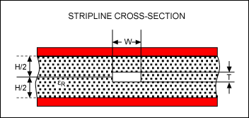
The Battle Against Signal Loss
At 5G frequencies, signals naturally weaken as they travel—this is insertion loss. On standard materials, loss can be 1–2 dB per foot at high frequencies. For a 10-inch trace, that could mean over 15 dB of loss, leaving the receiver with a signal too weak to detect.
To minimize loss:
- Go Short: Every unnecessary inch of trace adds loss. Route critical paths as directly as possible.
- Choose Premium “Pavement”: Use low-loss circuit board materials (e.g., specialized laminates). These can reduce signal loss by 40–60% compared to standard options.
- Shield the Highway: Ensure critical traces are flanked by solid ground planes. This contains the signal energy, preventing it from radiating away and causing further loss.
Rule 4: Route Differential Pairs Correctly—The DNA of Modern 5G Signaling
Why Differential Signaling Rules 5G
Differential signaling transmits information as the voltage difference between two complementary signals (P and N). This design choice is revolutionary:
- Common-mode noise rejection: If both P and N encounter the same noise (e.g., a power supply glitch), the difference (P − N) remains unchanged. Receivers, which measure only the difference, are immune to this common-mode noise.
- Smaller voltage swings needed: Differential signals achieve equivalent margins with 0.3–0.5V swings, reducing power consumption and EMI.
- Allows longer traces: Differential signals, with their common-mode immunity, can reliably propagate 1+ meters before requiring equalizers.
5G designs leverage differential signaling everywhere: SerDes interfaces (10–50 Gbps), DDR memory buses, RF modulation carriers. Almost every critical 5G path is differential.
Implementation Rules for Differential Pairs
Tight, consistent spacing: Route positive and negative traces with a center-to-center spacing of 0.3–0.5 mm (12–20 mils). Spacing that’s too tight (< 0.2 mm) makes routing congested; spacing that’s too loose (> 1 mm) breaks the differential coupling.
Equal trace length: P and N traces in a differential pair must be routed with equal length within ±2–5 mils. Length difference introduces differential skew—the two signals arrive at the receiver at slightly different times, reducing timing margin.
Minimize layer transitions: Every time a differential pair transitions between layers, there’s a brief moment where the coupling is lost. For critical pairs, keep layer transitions to a minimum (ideally ≤ 3 transitions).
Shielding ground traces or planes: On both outer edges of a differential pair, place a shielding trace connected to ground. These ground traces create a Faraday cage around the differential pair, preventing external noise from coupling in.
Via stitching around differential pairs: Along the length of a differential pair, place ground vias at 0.5–1 mm intervals. These vias ensure that any return currents have a short, low-inductance path directly to the reference plane.

Rule 5: Reduce Crosstalk with Spacing, Shielding, and Layer Strategy
Understanding the Two Types of Crosstalk
Capacitive crosstalk: Adjacent traces with different voltage transitions create transient electric fields that couple energy into neighboring traces. Magnitude: typically 50–150 mV for closely spaced traces.
Inductive crosstalk: A changing current in the aggressor trace creates a changing magnetic field; this field couples into the victim trace and induces a voltage proportional to the inductance and dI/dt. In a 5G system with edge rates of 200 mV/ns, even small mutual inductance creates significant inductive crosstalk—often 100–200 mV.
In tightly routed 5G boards, both mechanisms occur simultaneously, and crosstalk can easily exceed 250 mV on a single victim trace.

Crosstalk Mitigation Strategies
Aggressive trace spacing: 3W spacing (where W is trace width). For a 0.2 mm trace, this means 0.6 mm spacing. At this spacing, crosstalk typically decreases to 20–30 mV. For critical differential pairs, increase spacing further: 5W spacing (1.0 mm for a 0.2 mm trace) reduces crosstalk to < 10 mV.

Guard traces: Between critical trace pairs, route a guard trace (0.2–0.3 mm wide) connected to ground. This guard trace absorbs a portion of the coupling energy before it reaches the victim trace. Most effective when connected to the reference plane via stitching.
Via fences: A row of ground vias at 0.5–1 mm intervals along the length of a high-speed trace creates a Faraday cage that minimizes coupling to adjacent traces.
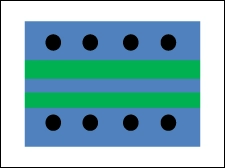
Layer strategy: Route high-speed and low-speed signals on different layers. Orthogonal routing is most effective: if the aggressor is routed east-west on Layer 3, route the victim north-south on Layer 4. Orthogonal routing reduces inductive coupling by 60–80%.
Rule 6: Design Solid Reference Planes and Ensure Clean Return Paths
The Critical Role of Return Paths in 5G Signal Integrity
Return currents are often overlooked—designers focus on forward signal routing while treating return paths as an afterthought. This is a catastrophic mistake. In high-speed designs, the loop inductance determines whether the design succeeds or fails.
For a simple single-ended signal routed over a 0.15 mm dielectric height to a ground plane 3 inches away, the loop inductance introduces ringing that consumes significant signal margin. When ground planes are fragmented, return currents are forced to detour around gaps, and loop inductance increases exponentially—potentially doubling or tripling, raising ringing from 50 mV to 150+ mV. This single design error can cause system failure.
Designing Robust Return Paths
Solid, continuous ground planes: Maintain unbroken ground planes on at least two layers. Never make exceptions: no cuts, no splits, no “strategic” isolated islands.

Via stitching for return path integrity: Along the length of every high-speed signal, place ground vias at intervals no greater than 1/20th of the signal wavelength. For a 5 GHz signal, this translates to approximately 1.5 mm via spacing. These vias minimize return path loop inductance; ringing is suppressed; crosstalk into adjacent traces is reduced.
Star grounding for mixed-signal circuits: In designs with both analog (RF front-end) and digital (baseband processor) sections, implement star grounding: connect all analog currents and all digital currents to a single point (the star) at which the connection to the board’s main ground plane occurs.
Power plane partitioning and return paths: Define ground regions for each voltage domain, and route all return vias for each voltage domain to its dedicated ground area. This prevents return current coupling between domains and keeps power supply noise localized.

Rule 7: Implement Disciplined Via Design for High-Speed and RF Nets
The Core Problem: Vias Can Degrade Your Signal
A via is the small plated hole that allows a signal to pass from one layer of the PCB to another. While necessary, every via acts like a tiny, unwanted circuit element—adding parasitic inductance and capacitance. For example, a typical via adds about 0.5–0.8 nH of inductance.
At 5G speeds, this small inductance creates a big problem: it becomes a significant impedance bump in the signal’s path. For a 5 GHz signal, this bump can cause roughly 33% of the signal energy to reflect. This reflection manifests as noise and distortion on the waveform, degrading signal integrity. Therefore, disciplined via design is about minimizing this disruptive effect.
Practical Techniques to Optimize Vias
You cannot avoid vias, but you can design them to be as “invisible” as possible to the signal. Here are key methods:
Use Multiple Vias for Power and Ground: A single via has fixed inductance. For power and ground connections, use several vias in parallel (e.g., an array of 4). This divides the inductance among them, significantly lowering the total impedance for stable power delivery.
Use Back-Drilling to Remove Stubs: A standard via goes through all layers, creating an unused conductive “stub” beyond the target layer. Back-drilling uses a second drill operation to remove this stub. Result: via inductance is reduced by 30–40%, and reflections are cut by about 50%. This is highly recommended for critical RF paths.

Consider Blind or Buried Vias in Dense Designs: A blind via connects an outer layer to an inner layer without going through the entire board. A buried via connects inner layers only. Both eliminate long stubs, minimizing parasitics and saving space. They cost more but are often essential for compact, high-performance 5G modules.
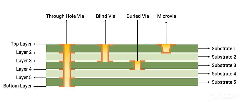
Place Vias Directly in Pads (Via-in-Pad): For components like BGAs, place the via directly in the component’s solder pad. This minimizes the connecting trace and its associated inductance. Result: This can reduce via-related inductance by another 30–40% and improve impedance matching.

Control Impedance Through Via Geometry: Work with your PCB manufacturer to design the via structure—specifically the pad and anti-pad sizes—based on your stack-up. The goal is to minimize the impedance discontinuity at the transition. For instance, a 0.23 mm trace might require a carefully calculated via pad and a specific anti-pad diameter in the surrounding plane to keep impedance as close to 50Ω as possible through the via.
Rule 8: Maintain Power Integrity with Proper Decoupling, Placement, and Supply Rail Design
Why Power Integrity Is Signal Integrity
A 5G transceiver SoC with hundreds of logic gates switching simultaneously can exhibit transient supply current spikes of 10–20A. If the power delivery network (PDN) has excessive impedance, the voltage droop across that impedance becomes problematic, pushing signal thresholds lower and reducing timing margin.
Power integrity is therefore inseparable from signal integrity. A design with good clock routing but poor PDN will fail because the low power supply ruins the clock distribution.
Decoupling Strategy: A Hierarchical Approach
The modern PDN uses a hierarchy of capacitor values to address different frequency ranges:
| Capacitor Value | Frequency Range | Primary Role | Typical Quantity (per 200-pin SoC) |
|---|---|---|---|
| 0.1 µF | 100 MHz – 1 GHz | High-frequency transient current absorption | 50–100 pcs |
| 1 µF | 10–100 MHz | Mid-frequency ripple smoothing | 20–30 pcs |
| 10 µF | 1–10 MHz | Low-frequency sagging absorption | 5–10 pcs |
| Bulk (100 µF+) | < 1 MHz | Low-frequency supply regulation | 2–5 pcs |
Placement discipline for decoupling capacitors: Place all 0.1 µF capacitors within 5 mm of their associated power pin. At this distance, the trace inductance is minimized, and the capacitor effectively bypasses high-frequency noise. Longer traces introduce unwanted series inductance, reducing the capacitor’s effectiveness.
Distribute capacitors evenly around the device perimeter. Clustering all capacitors on one side creates local current congestion and uneven voltage distribution.

Power plane copper distribution: Dedicate continuous copper layers to 3.3V, 1.8V, and 0.9V power supplies (in addition to ground planes). Power planes offer a distributed capacitive effect—the FR-4 dielectric between the power and ground planes acts as a massive capacitor. This distributed capacitance, combined with the low inductance of the parallel structure, provides broadband impedance reduction.
Supply rail trace design: Power distribution traces should be wide and short. Avoid long, thin power traces.
Rule 9: Validate with Simulation and Post-Layout Measurements Before Prototype Commitment
Pre-Layout Simulation: Your First Line of Defense
Before committing to fabrication, validate critical signal paths using electromagnetic simulation. Modern tools compute characteristic impedance, eye diagrams, jitter, and S-parameters.
Simulation catches 80% of signal integrity problems before fabrication. The remaining 20% require physical validation on prototypes.
Post-Layout Measurement Methodology
Once the prototype arrives, validate with three key measurements:
Time-Domain Reflectometry (TDR): Inject a fast transient into a trace and measure reflections. TDR reveals impedance discontinuities, stub effects, and vias. A well-designed trace shows a smooth impedance profile with minimal reflections.
Network analyzer measurement: Measure S-parameters across the frequency range of interest. Return loss should exceed –20 dB, indicating excellent impedance matching. Insertion loss should align with pre-layout simulation predictions.
Oscilloscope waveform capture: Route test traces to BNC connectors. Connect a high-bandwidth oscilloscope (bandwidth ≥ 3× signal frequency) and capture actual voltage waveforms under real operating conditions.
Common Failure Signatures and Remedies
| Symptom | Root Cause | Quick Verification | Remedy |
|---|---|---|---|
| Excessive ringing | Impedance mismatch | TDR shows ±15%+ variation | Adjust trace width |
| Intermittent bit errors | Tight timing margin | Measure clock jitter | Reduce trace skew |
| Crosstalk-induced noise | Insufficient spacing | Network analyzer shows S12 > –25 dB | Increase spacing |
| Thermal failures | Inadequate power delivery | Measure VDD ripple | Add capacitors |
| Signal loss | Inadequate material selection | Measure insertion loss | Switch to low-loss material |
Rule 10: Collaborate with Your PCB Manufacturer from Design Inception
Why Design-Manufacturing Partnership Matters
The gap between an electrically beautiful design and a manufacturable design is often larger than expected. Working with your PCB manufacturer from day one prevents design rework and cost surprises.
Early Collaboration Checklist
Week 1–2: Stackup Review
Share your signal integrity plan and target stackup with the manufacturer. Confirm material availability and lead time before committing to the design.
Week 3–4: Design Rule Definition
The manufacturer provides standard design rules. You confirm which rules can be relaxed and which are inviolable.
Week 5–8: Layout Review
Submit preliminary Gerber files for DFM (Design for Manufacturability) review. Identify issues before committing to fabrication.
Week 9: Sample Board Inspection
Order 5–10 prototype boards and request detailed process data: layer stackup cross-section, impedance coupon measurements, insertion loss measurements, and copper surface roughness.
Design Information to Provide Manufacturers
Signal Integrity Plan: One-page document specifying target impedance, frequency band, loss budget, and margin requirements.
Layer Stackup Drawing: Material specifications, layer names, copper weights, dielectric thickness, via specifications.
Design Rules Document: Specification of trace width, spacing, via diameter, and pad clearances.
Test Point Locations: Coordinates for oscilloscope measurement points, impedance coupons, and DFT access points.
Common 5G PCB Signal Integrity Pitfalls to Avoid
Pitfall 1: Underestimating Crosstalk in Dense Layouts
Problem: Designers assume crosstalk is negligible if trace spacing meets design rules. Reality: at 5G frequencies, inadequate spacing introduces 100–200 mV of coupling.
Prevention: Measure actual crosstalk on prototypes using a network analyzer.
Pitfall 2: Fragmented or Split Ground Planes
Problem: Designers route signal traces “around” ground plane regions rather than over them. Return currents detour, increasing loop inductance.
Prevention: Enforce a rule: “No high-speed signals route across split ground planes.”
Pitfall 3: Inadequate Via Stitching or Inconsistent Spacing
Problem: Via stitching spacing is inconsistently applied. Some regions have 0.5 mm stitching; others have 2 mm spacing.
Prevention: Use design rule checks (DRC) in your CAD tool to automatically verify via stitching spacing.
Pitfall 4: Optimizing for Impedance While Ignoring Insertion Loss
Problem: Designers carefully control impedance but use standard FR-4 without considering loss.
Prevention: Calculate expected insertion loss for signal paths before finalizing material selection.
Pitfall 5: Placing All Decoupling Capacitors on One Side
Problem: A 200-pin SoC with all decoupling capacitors placed on one side exhibits higher power supply noise on the opposite side.
Prevention: Distribute capacitors evenly around device perimeter.
Pitfall 6: Ignoring Temperature Coefficients of Impedance and Dk
Problem: Impedance and dielectric constant change with temperature. PCB material Dk might shift from 4.3 at 25°C to 4.5 at 85°C, shifting impedance by 5%.
Prevention: Simulate designs at temperature extremes. Design with ±10% impedance tolerance rather than ±5%.
Material Selection and Stack-Up Summary Table
| Design Target | Frequency Range | Recommended Material | Dk Value | Df (Dissipation) | Cost vs. FR-4 | Comments |
|---|---|---|---|---|---|---|
| Standard Wireless | < 2.4 GHz | Standard FR-4 | 4.3 | 0.025 | 1× | Cost-effective |
| 5G Sub-6 GHz | 3–6 GHz | Low-loss FR-4 or hydrocarbon | 4.3 or 3.5 | 0.008 | 1.2–1.5× | Loss reduction critical |
| 5G Mid-Band | 24–28 GHz | Rogers RO4835 | 3.5 | 0.004 | 1.5–2.0× | Mandatory for acceptable loss |
| 5G mmWave | 26–100 GHz | PTFE-based (Rogers) | 3.0–3.5 | < 0.002 | 2.0–3.0× | Low loss mandatory |
How IWDF Solutions Helps You Implement These 10 Golden Rules
Our Role as Your PCB Engineering Partner
At IWDF Solutions, we are a specialized Shenzhen-based PCB design, reverse engineering, and PCBA manufacturing partner serving global 5G equipment manufacturers. Over the past decade, we’ve completed 500+ production-volume 5G PCB designs, processing over 2.5 million units annually.
Early-Stage Collaboration: Stack-Up and Material Selection
You provide: Block diagram, target frequency bands, data rates, and power budget.
We deliver: Stackup recommendations, material comparison, preliminary design rules, and risk assessment.
Layout Support and DFM Review
You provide: Preliminary Gerber files, net list, and stackup definition.
We perform: Critical path analysis, signal integrity simulation, and DFM assessment.
We deliver: Specific recommendations for impedance improvement via optimization, trace routing corrections.
Prototype Fabrication and Validation
You provide: Final Gerber files, test requirements.
We deliver:
- Fabrication with impedance control and stackup verification
- TDR and network analyzer measurement on critical paths
- Layer cross-section analysis confirming copper weights
- Thermal imaging under load
- Full functional testing under temperature variation
Production Ramp with Continued Support
You provide: Approved prototype, long-term volume forecast.
We ensure:
- Consistent process parameters and material lot control
- Ongoing impedance and test coupon measurement
- Traceability documentation for each production batch
- Rapid response to any in-field issues
Our Technical Advantages
In-house capability: We maintain laboratory equipment and signal integrity simulation software.
Experience: Our engineering team has 12+ years of average experience in high-speed design.
Process control: Our facility is ISO 9001:2015 and IPC-A-610 Class 3 certified.
FAQ: Signal Integrity and 5G Design
Q1: Can I design a 5G sub-6 GHz board using standard FR-4?
A: Technically yes, but with constraints. Standard FR-4 is acceptable for sub-6 frequencies if your link budget can tolerate 3–4 dB of insertion loss per 12 inches.
Q2: How many ground planes do I really need?
A: Minimum 2 (Layers 2 and 6). Ideally, 3 (Layers 2, 6, and 9). Focus on placement (adjacent to high-speed signals) rather than raw quantity.
Q3: What’s the optimal via stitching spacing for 5G designs?
A: Target 1/20th of the signal wavelength at your highest frequency. For 5 GHz, approximately 1.5 mm. For 28 GHz, approximately 0.3 mm. In practice, 0.5–1 mm spacing is good for sub-6 GHz; 0.3–0.5 mm for mmWave.
Q4: Should I use back-drilling on every via?
A: No. Back-drill only critical vias (clocks, high-speed SerDes > 10 Gbps). For moderate-speed signals (< 5 Gbps), back-drilling provides diminishing returns.
Q5: How do I know if my impedance control is adequate?
A: Measure actual impedance on prototypes using TDR. If measured impedance is within ±10% of the target, you’re good.
Q6: What’s the practical minimum trace-to-trace spacing for 5G designs?
A: Standard manufacturing capability: 0.1 mm (4 mils). For high-volume production, design to 0.15 mm (6 mils).
Q7: Do I need separate analog and digital ground planes?
A: Not necessarily. Implement star grounding—merge all return currents at a single point.
Q8: How does temperature affect signal integrity?
A: PCB material Dk and Df shift with temperature. Design to ±10% impedance tolerance (rather than ±5%) to accommodate temperature variation.
Q9: When should I use differential signaling vs. single-ended?
A: Differential for: high-speed clocks (> 1 GHz), high-speed serial (> 5 Gbps), long traces (> 30 cm). Single-ended for: moderate speeds (< 500 Mbps), short distances (< 10 cm).
Q10: What simulation tools do I need for 5G PCB design?
A: At minimum: an impedance calculator (field solver). Strongly recommended: transmission line simulator. Optional but valuable: full-wave electromagnetic simulator.
Conclusion: Transforming 5G Design Complexity Into Confidence
These ten golden rules transform signal integrity from an arcane afterthought into a systematic, reproducible engineering discipline. When applied rigorously, they:
- Reduce rework by 60%: First-pass design success rates improve dramatically.
- Improve manufacturing yield by 40%: Designs optimized for both electrical performance and manufacturability yield fewer defects.
- Accelerate time-to-market by 8–12 weeks: Fewer iteration cycles and faster certification enable faster product launch.
- Build customer trust: Products that “just work”—without intermittent failures or thermal sensitivity—establish market leadership.
5G PCB design is admittedly complex. But complexity is predictable if you follow a proven framework.
Your role is to establish clear electrical objectives, select materials and stackup thoughtfully, implement routing discipline rigorously, and validate relentlessly. Our role, as your PCB manufacturing partner, is to ensure that your vision translates faithfully into physical boards that meet or exceed your electrical targets.
If you’re designing or manufacturing a 5G module, antenna, transceiver, or edge device and need a partner who genuinely understands the intersection of signal integrity and manufacturing reality, we’re here to help. We’ve been in the trenches on 500+ designs and thousands of debugging sessions.
Let’s build reliable, market-winning 5G products together. Contact us!